The support vector machine (SVM) is a very different approach for supervised learning than decision trees. In this article I will try to write something about the different hyperparameters of SVM.

Different kernels

The main hyperparameter of the SVM is the kernel. It maps the observations into some feature space. Ideally the observations are more easily (linearly) separable after this transformation. There are multiple standard kernels for this transformations, e.g. the linear kernel, the polynomial kernel and the radial kernel. The choice of the kernel and their hyperparameters affect greatly the separability of the classes (in classification) and the performance of the algorithm.

The linear kernel

The linear kernel is $K(x_i, x_j) = x_i’ x_j$.

When using this kernel we only have one hyperparameter in SVM: The cost parameter $C$.

The polynomial kernel

The polynomial kernel is $K(x_i, x_j) = (r + \gamma \cdot x_i’ x_j)^d$.

Usually the parameter $r$ is set to zero and $\gamma$ to a fixed value, e.g. $1/n$ with $n$ being the number of observations. Beside the cost parameter $C$ the integer parameter $d$ has to be tuned, usually values between 1 and 10 are chosen.

The radial kernel

The radial kernel is $K(x_i, x_j) = e^{\gamma \cdot x_i’ x_j}$.

This kernel is the most used and most successful kernel, due to the flexibility of separating observations with this method. Additionally to the cost parameter $C$, the hyperparameter $\gamma$ has to be tuned. In the paper A practical guide to Support Vector Classifier they recommend to search $C$ in the range $[2^{-5}; 2^{15}]$ and $\gamma$ in the range $[2^{-15};2^3]$.

Tuning of the radial kernel in R

Tuning in R can be done easily with the mlrHyperopt R package, which is based on mlr and mlrMBO.

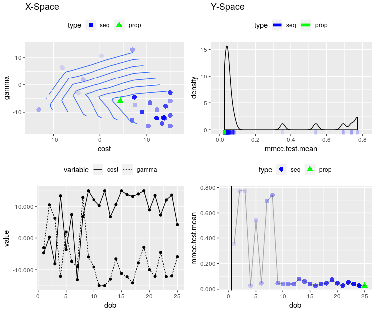
In the following we can see the tuning of SVM with radial kernel (tuning parameter $C$ and $\gamma$) for the iris classification task.

devtools::install_github("berndbischl/ParamHelpers") # version >= 1.11 needed.
devtools::install_github("jakob-r/mlrHyperopt", dependencies = FALSE)

library(mlrHyperopt)
res = hyperopt(iris.task, learner = "classif.svm")
res
# Tune result:
# Op. pars: cost=1.21e+04; gamma=0.000239
# mmce.test.mean=0.0266667

With plotOptPath we can see a picture of the performance of SVM dependent on the two hyperparameters and some other informations of the tuning process:

plotOptPath(res$opt.path)

It is also possible to use mlrHyperopt within mlr, by using a Wrapper. Then all the tools and possibilities that are available in the mlr package can be used. Here is an example code:

task = makeClassifTask(data = iris, target = "Species")
lrn = makeLearner("classif.svm")
lrn = makeHyperoptWrapper(lrn)
mod = train(lrn, task)
print(getTuneResult(mod))
# Tune result:
# Op. pars: cost=42.6; gamma=0.0084
# mmce.test.mean=0.0333333

Instead of using model-based optimization for tuning other tuning strategies especially tailored for SVM can be used. This will be the topic of one of the following blog posts.